Degree Distribution Analysis

What is Degree Distribution?

• Vertex Degree: In a network (or a graph), each node (or vertex) has a certain number of connections to other nodes. The number of connections a node possesses is called its degree.
• Degree Distribution: The degree distribution of a network provides a picture of how these degrees are spread out across the nodes. It essentially tells you how many nodes have one connection, how many have two connections, and so on.

Types of Degree Distributions

There are several common types of degree distributions, each telling us something different about the structure of the network:

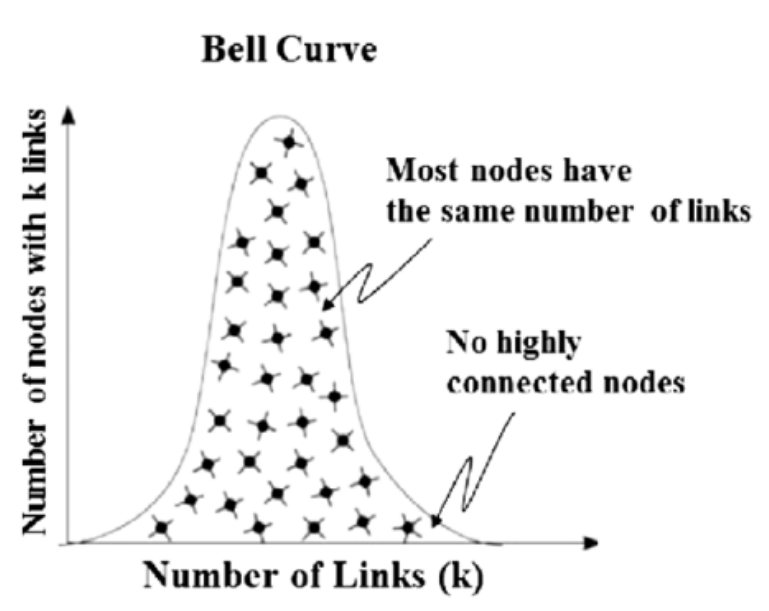
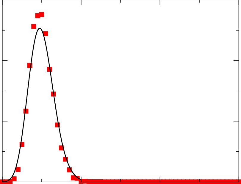
• Random Networks: These exhibit a bell-shaped distribution (similar to a normal distribution) where most nodes have a degree close to the average. Imagine a group of people where each person randomly knows a few others. Most people would have a similar number of friends.

• Scale-free Networks: These are characterized by a power-law distribution–a few nodes have an exceptionally high number of connections (these are called “hubs”) while the majority of nodes have very few connections.
  Think of a social media platform. A few users (influencers) have thousands of followers, while most users have relatively few. The degree distribution has a long tail, indicating the presence of hubs.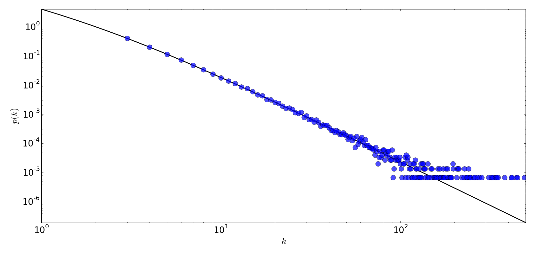

• Small-world Networks: These display a combination of high clustering (nodes tend to form tightly knit groups) and short average path lengths (you can get from one node to another relatively quickly).

Imagine a friend group where everyone knows most of the same people (high clustering), but there are always a few ‘connectors’ who bridge different groups (short average distance).

The degree distribution has a narrower peak than a random network, but might still show a slightly longer tail.

Interpreting the Distribution

Imagine analyzing the friend network we talked about early. Those degree distributions could tell us:

Mostly even distribution (bell-shaped): People tend to have a similar number of friends, with no clear ‘super-connectors’. This could indicate a more niche platform with less focus on influencers.

Long, heavy tail: Classic sign of a scale-free network—a few users have vastly more connections. The platform likely relies heavily on influencers for content and reach.

Clustered but short distances: This suggests a small-world network, where most users are connected within groups but can easily reach others outside their circle. This might indicate a high potential for information to spread quickly.

But how to actually perform degree distribution analysis?

1. Data Collection: First, you need data representing your network. This is often in the form of an adjacency list or adjacency matrix(check out my next post to learn more), which shows the connections between nodes.
2. Calculate Degrees: For each node in your network, count the number of edges (connections) it has. This gives you the degree of each node(Gephi and NetwrokX can do this).
3. Create Distribution: Tally up the number of nodes that exist for each degree value. For example, how many nodes have a degree of 1, how many have a degree of 2, and so forth.
4. Visualization: Plot this information as a histogram or a line graph. The x-axis will represent the degrees, and the y-axis will represent the number of nodes at each degree.

Applications

Degree distribution analysis has a wide range of applications across different fields:

• Social Networks: Analyzing patterns of friendships or followers to understand the spread of information, trends, and influence.
• Computer Networks: Evaluating the structure of the internet and its vulnerability to failures or attacks.
• Biology: Studying protein interaction networks to understand the importance of certain proteins in biological processes.
• Epidemiology: Modeling the spread of diseases based on contact patterns within a population.

Specific Practicle Examples with NetworkX

NetworkX is a powerful Python library for creating, manipulating, and analyzing networks(We talked about it in early post). Here’s how we can use it for degree distribution analysis on some examples:

1. Social Network (Scale-free)

import networkx as nx
import matplotlib.pyplot as plt

# Create a scale-free network using the Barabasi-Albert model
G = nx.barabasi_albert_graph(n=1000, m=2)  # 1000 nodes, each node attaches to 2 existing nodes

# Calculate degree for each node
degrees = [G.degree(node) for node in G.nodes()] 

# Plot the degree distribution
plt.hist(degrees)
plt.xlabel("Degree")
plt.ylabel("Number of Nodes")
plt.title("Degree Distribution of a Scale-Free Network")
plt.show()

Important Note: You’ll need datasets to represent your network (e.g., edge lists). NetworkX supports many common formats.

A short introduction on network data

• Edge Lists: One of the simplest formats. This is a text file where each line represents an edge (connection) between two nodes.
  • Example:

    Node1 Node2
    Node2 Node5
    Node1 Node3
    

• Adjacency Matrices: A matrix where rows and columns represent nodes. A value in a cell indicates if an edge exists between the corresponding pair of nodes.

• Specialized Formats:
  • GraphML: An XML-based format for flexible network representation.
  • GEXF: Another XML format, often used for dynamic and hierarchical networks.
  • Shapefiles (for geospatial networks): Used to represent roads, power lines, etc. Requires libraries like GeoPandas.

Sources of Network Datasets

1. Public Repositories:
   • Stanford Large Network Dataset Collection (SNAP): https://snap.stanford.edu/data/ (Social networks, web graphs, etc.)
   • Network Repository: http://networkrepository.com/ (Various domains)
2. Real-world Data Collection:
   • Social Media APIs: Extract follower/friendship networks(See APIs post in General).
   • Web Scraping: Build networks by crawling links on websites (proceed ethically).
   • Scientific Datasets: Collaboration networks, protein interactions, etc.
3. Synthetic Data Generation:
   • NetworkX provides models for creating random graphs, scale-free networks, etc. This is useful for experimentation and simulations.

Working with Datasets in NetworkX

• Loading Network Data:
  • Edge lists: nx.read_edgelist("your_file.txt")
  • Adjacency lists: nx.read_adjlist("your_file.txt")
  • GraphML, GEXF, etc.: NetworkX supports these formats as well.
• GIS Datasets:
  • You’ll likely need GeoPandas to load shapefiles and then convert them into suitable NetworkX graph representations.

Important Considerations

• Data Cleaning: Real-world data often requires preprocessing to handle missing values, inconsistencies, and proper formatting.
• Choice of Format: The format you choose depends on your data source and the type of analysis you intend to perform.
• Spatial Networks: Handling geographic networks may necessitate additional geospatial libraries.